Nothing in this article should be considered as investment advice
Overview
In the US, publicly traded companier are required to publish an annual report, called a 10-K. In addition to basic financial information, these reports include management commentary and a disclosure of perceived risks. While the financials are typically where analysts focus, attention is given to reading between the lines of the typically bland and risk adverse narrative sections.
I got interested in using R to automate the process of grabbing the 10K from the SEC website, parsing out the narrative sections, and applying basic sentiment and text analysis.
Basics
It was working on this project that led to the creation of the edgarWebR package and we’ll be using it extensively as we look up a company, find its annual filings, and fetching the management report.
First, we’ll specify the ticker we’re interested in and the number of years we want to analyze. Using that we can find the company information.
ticker <- 'EA'
years <- 5
company.details <- company_details(ticker, type = "10-K", count = years)

#TODO: better formatting company information**
kable(company.details$information %>% select(name, cik, fiscal_year_end),
col.names=c('Company Name', 'CIK', 'Fiscal Year End'))| Company Name | CIK | Fiscal Year End |
|---|---|---|
| ELECTRONIC ARTS INC. | 0000712515 | 0331 |
Next, look up reports in the SEC EDGAR system and look in each filing to find the report. A lot is happening in a few lines, but effectively we’re going from a list of annual filings to urls for the main document in each filing.
One note - while, we specified both the type (10-K) and count (5), because the SEC site isn’t precise, we need to re-filter.
# Each filing is made up of multiple documents,
# this extracts the main narrative
filing_doc <- function(href) {
  sapply(href, function(x) {
         filing_documents(x) %>%
         filter( type == "10-K" ) %>% select(href) }) %>%
  unlist(recursive = TRUE, use.names = FALSE)
}
company.reports <- company.details$filings %>%
  filter(type == "10-K") %>%
  slice(1:years) %>%
  mutate(doc.href = filing_doc(href),
         mdlink = paste0("[Filing Link](", href, ")"),
         reportLink = paste0("[10-K Link](", doc.href, ")")) %>%
  select(filing_date, accession_number, mdlink, reportLink, href, doc.href)

knitr::kable(company.reports %>% select(-href, -doc.href),
col.names=c('Filing Date', 'Accession #', 'Filing Link', '10-K Link'))| Filing Date | Accession # | Filing Link | 10-K Link |
|---|---|---|---|
| 2018-05-23 | 0000712515-18-000024 | Filing Link | 10-K Link |
| 2017-05-24 | 0000712515-17-000035 | Filing Link | 10-K Link |
| 2016-05-27 | 0000712515-16-000111 | Filing Link | 10-K Link |
| 2015-05-21 | 0000712515-15-000033 | Filing Link | 10-K Link |
| 2014-05-21 | 0000712515-14-000024 | Filing Link | 10-K Link |
We now have a link to the narrative 10-K for each of the past 5 years.
Parse out 10K
To perform sentiment analysis, the next big step is to take the HTML formatted 10-K and turn it into a set of words. While we won’t use it right now, we’ll also parse the various sections of the document for later filtering.
Warning: this gets hairy…
knitr::spin_child("../R/parse10k.R")
parse10k <- function(uri) {
  # 10-K HTML files are very flat with a long list of nodes. This pulls all
  # the relevant nodes.
  nodes <- read_html(uri) %>% html_nodes('text') %>% xml_children()
  nodes <- nodes[xml_name(nodes) != "hr"]

  # Unfortunately there isn't much of a workaround to this loop - we need
  # to track position in the file so it has to be a bit sequential...
  doc.parts <- tibble(nid = seq(length(nodes)),
                     node = nodes,
                     text = xml_text(nodes) ) %>%
              filter(text != "") # way to get columns defined properly

  parts <- doc.parts %>%
    filter(grepl("^part",text, ignore.case=TRUE)) %>%
    select(nid,text)
  #  mutate(next.nid = c(nid[-1],length(nodes)+1)) %>%
  if (parts$nid[1] > 1) {
    parts <- bind_rows(tibble(nid = 0, text= "PART 0"), parts)
  }
  parts <- bind_rows(parts,
                     tibble(nid = doc.parts$nid[length(doc.parts$nid)] + 1,
                            text = "NA"))

  items <- doc.parts %>%
    filter(grepl("^item",text, ignore.case=TRUE)) %>%
    select(nid,text) %>%
    mutate(next.nid = c(nid[-1],length(nodes)+1),
           part.next = parts$nid[findInterval(nid,parts$nid) + 1],
           next.nid = ifelse(part.next < next.nid, part.next, next.nid),
           prev.end = c(0,next.nid[-length(nid)]))

  # Fill in item gaps w/ N/A
  n <- 0
  for(i in seq(length(items$nid))) {
    j <- i + n
    if(items$prev.end[j] != items$nid[j]) {
      items <- items %>%
        add_row(nid = items$prev.end[j], text = NA, .before = j)
      n <- n + 1
    }
  }

  doc.parts <- doc.parts %>%
    mutate( part = parts$text[findInterval(nid, parts$nid)],
            item = items$text[findInterval(nid, items$nid)]) %>%
    select(nid,part,item,text)

  return(doc.parts)
}
We then take our parsing function and run it against each of the reports
data <- company.reports %>% rowwise() %>%
  mutate(nodes = map(doc.href, parse10k)) %>%
  select(-accession_number, -href, -mdlink, -doc.href, -reportLink) %>%
  ungroup() %>%
  group_by(filing_date)
Finally, we use unnest_tokens from TidyText to prepare our documents for sentiment analysis
words <- data %>%
  unnest(nodes) %>%
  select(-nid) %>%
  unnest_tokens(word, text)
words
## # A tibble: 261,407 x 4
## # Groups: filing_date [5]
## filing_date part item word
## <dttm> <chr> <chr> <chr>
## 1 2018-05-23 00:00:00 PART 0 <NA> document
## 2 2018-05-23 00:00:00 PART 0 <NA> united
## 3 2018-05-23 00:00:00 PART 0 <NA> states
## 4 2018-05-23 00:00:00 PART 0 <NA> securities
## 5 2018-05-23 00:00:00 PART 0 <NA> and
## 6 2018-05-23 00:00:00 PART 0 <NA> exchange
## 7 2018-05-23 00:00:00 PART 0 <NA> commission
## 8 2018-05-23 00:00:00 PART 0 <NA> washington
## 9 2018-05-23 00:00:00 PART 0 <NA> d.c
## 10 2018-05-23 00:00:00 PART 0 <NA> 20549
## # ... with 261,397 more rowsWe can also use this to run a quick wordcloud!
words %>%
  ungroup() %>%
  anti_join(stop_words) %>%
  ungroup() %>%
  count(word) %>%
  with(wordcloud(word,n,max.words = 75, use.r.layout=FALSE, rot.per=0.35))
## Joining, by = "word"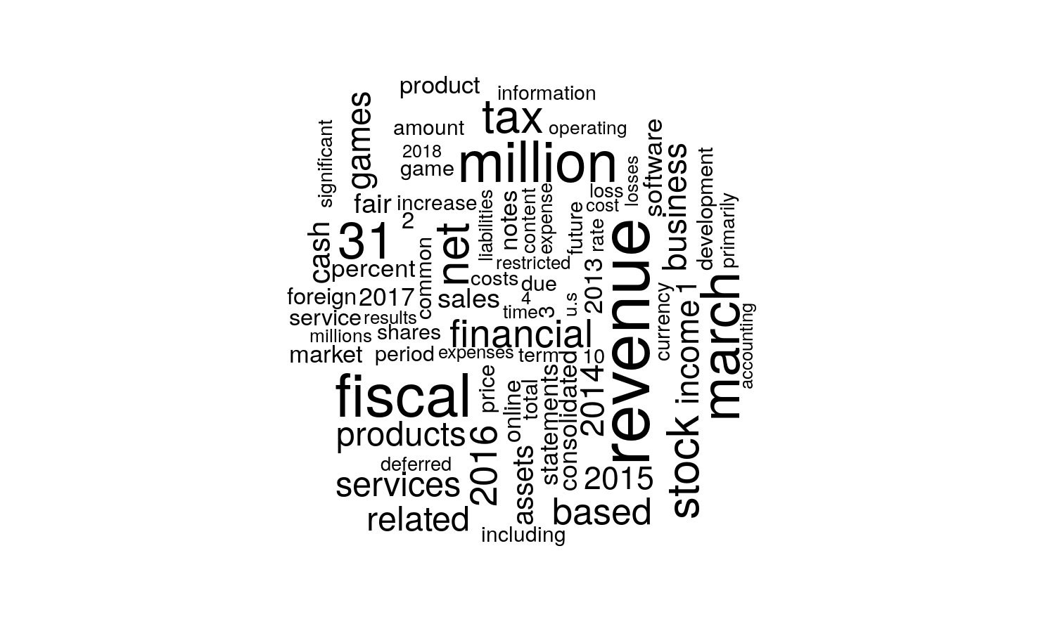
Basic Sentiment Analysis
Basic sentiment analysis just assigns a sentiment to each word, so getting the sentiment of a particular document just requires adding up the sentiments. There are a lot of sentiment data sets included in tidytext, but for this proof of concept, we’ll use the simplest (and most widely used), bing. The bing lexicon assigns each word to be positive, negative or neutral.
Following the process outlined by Text Mining with R, we compute a sentiment for each filing.
word.counts <- words %>%
  group_by(filing_date) %>%
  summarize(words = n())

bing <- words %>%
  inner_join(get_sentiments("bing"), by=c("word")) %>%
  count(filing_date, sentiment) %>%
  spread(sentiment,n,fill=0) %>%
  left_join(word.counts, by=("filing_date")) %>%
  mutate(sentiment = positive-negative,
         sentiment.ratio = sentiment/words,
         positive.ratio = positive/words,
         negative.ratio = negative/words ) %>%
  filter(TRUE) # Noop so we can comment things in the middle for testing
ggplot(bing, aes(x=filing_date, y=sentiment)) +
  geom_col() +
  labs(x='Filing Date', y='Sentiment', title='10-K Sentiment')
knitr::kable(bing,
  col.names=c('Filing Date', "Neg.", "Pos.", 'Total Words', 'Sentiment',
'Sentiment Ratio', 'Pos. Ratio', 'Neg. Ratio'))| Filing Date | Neg. | Pos. | Total Words | Sentiment | Sentiment Ratio | Pos. Ratio | Neg. Ratio |
|---|---|---|---|---|---|---|---|
| 2014-05-21 | 949 | 1150 | 58383 | 201 | 0.0034428 | 0.0196975 | 0.0162547 |
| 2015-05-21 | 911 | 1073 | 53697 | 162 | 0.0030169 | 0.0199825 | 0.0169656 |
| 2016-05-27 | 906 | 1004 | 51284 | 98 | 0.0019109 | 0.0195773 | 0.0176663 |
| 2017-05-24 | 819 | 908 | 47719 | 89 | 0.0018651 | 0.0190281 | 0.0171630 |
| 2018-05-23 | 879 | 1006 | 50324 | 127 | 0.0025236 | 0.0199905 | 0.0174668 |
Discussion
A cursory glance suggests something interesting might be going on, with an apparent decline in sentiment over the preceding 5 years. It is important to point out a few limitations for the current level of analysis -
- Use of a general sentiment lexicon - There are financial specific sentiment lexicons that would be more appropriate. e.g. in the financial context, ‘gross’ is fairly neutral, as in ‘gross receipts’.
- Whole report analysis - There is a lot of material in a 10-K but for sentiment analysis we likely only want Management’s Report and Risks.
- Relative comparison - Without comparing these results to other companies and their financials, it is impossible to say if this drop is statistically significant.
I’ll be addressing all of these in future posts and comparing report sentiment to financial results.
While only a first step, we’ve managed to fully programaically go from a ticker symbol to a multi-year sentiment analysis, opening up a lot of interesting possibilities.